Abstract
The 2013–2016 epidemic of Ebola virus disease was of unprecedented magnitude, duration and impact. Analysing 1610 Ebola virus genomes, representing over 5% of known cases, we reconstruct the dispersal, proliferation and decline of Ebola virus throughout the region. We test the association of geography, climate and demography with viral movement among administrative regions, inferring a classic ‘gravity’ model, with intense dispersal between larger and closer populations. Despite attenuation of international dispersal after border closures, cross-border transmission had already set the seeds for an international epidemic, rendering these measures ineffective in curbing the epidemic. We address why the epidemic did not spread into neighbouring countries, showing they were susceptible to significant outbreaks but at lower risk of introductions. Finally, we reveal this large epidemic to be a heterogeneous and spatially dissociated collection of transmission clusters of varying size, duration and connectivity. These insights will help inform interventions in future epidemics.
At least 28,646 cases and 11,323 deaths1 have been attributed to the Makona variant of Ebola virus (EBOV)2 in the two and a half years it circulated in West Africa. The epidemic is thought to have begun in December 2013 in Guinea, but was not detected and reported until March 20143. Initial efforts to control the outbreak in Guinea were considered to be succeeding4, but in early 2014 the virus crossed international borders into neighbouring Liberia (first cases diagnosed in late March) and Sierra Leone (first documented case in late February5, 6, first diagnosed cases in May7). EBOV genomes sequenced from three patients in Guinea early in the epidemic3 demonstrated that the progenitor of the Makona variant originated in Middle Africa and arrived in West Africa within the last 15 years7, 8. Rapid sequencing from the first reported cases in Sierra Leone confirmed that EBOV had crossed the border from Guinea and were not the result of an independent zoonotic introduction7. Subsequent studies analysed the genetic makeup of the Makona variant, focusing on Guinea9–11, Sierra Leone12, 13 or Liberia14, 15, identifying local viral lineages and transmission patterns within each country.
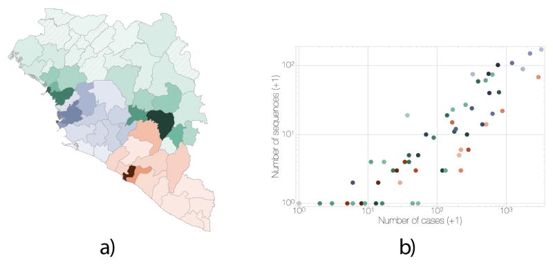
Although virus sequencing has covered considerable fractions of the epidemic in each affected country, individual studies focused on either limited geographical areas or time periods, so that the regional level patterns and drivers of the epidemic across its entire duration have remained uncertain. Using 1610 genome sequences collected throughout the epidemic, representing over 5% of recorded Ebola virus disease (EVD) cases (Figure 1), we reconstruct a detailed phylogenetic history of the movement of EBOV within and between the three most affected countries. Using a recently developed phylogeographic approach that integrates covariates of spatial spread16, we test which features of each region (administrative, economic, climatic, infrastructural and demographic) were important in shaping the spatial dynamics of EVD. We also examine the effectiveness of international border closures on controlling virus dissemination. Finally, we investigate why regions that immediately border the most affected countries did not develop protracted outbreaks similar to those that ravaged Sierra Leone, Guinea and Liberia.
Figure 1. Distribution and correlation of EVD cases and EBOV sequences.
a) Administrative regions within Guinea (green), Sierra Leone (blue) and Liberia (red); shading is proportional to the cumulative number of known and suspected EVD cases in each region. Darkest shades represent 784 cases for Guinea (Macenta Prefecture), 3219 cases for Sierra Leone (Western Area Urban District) and 2925 cases for Liberia (Montserrado County); hatching indicate regions without reported EVD cases. Circle diameters are proportional to the number of EBOV genomes available from that region over the entire EVD epidemic with the largest representing 152 sequences. Crosses mark regions for which no sequences are available. Circles and crosses are positioned at population centroids within each region. b) A plot of number of EBOV genomes sampled against the known and suspected cumulative EVD case numbers. Regions in Guinea are denoted in green, Sierra Leone in blue and Liberia in red. Spearman correlation coefficient: 0.93.
Origin, ignition and trajectory of the epidemic
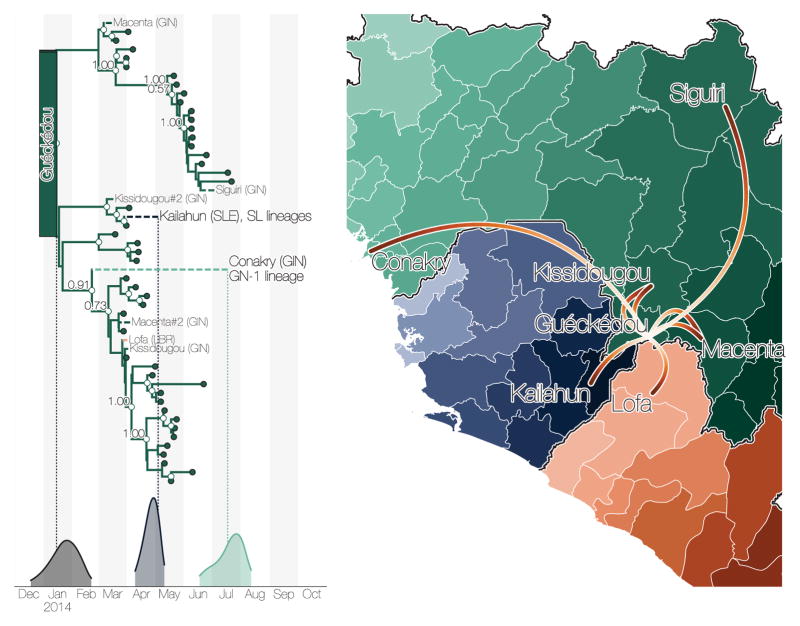
Molecular clock dating indicates that the most recent common ancestor of the epidemic existed between December 2013 and February 2014 (mean 2014.06, 95% credible interval, CI: 2013.96, 2014.14) and phylogeographic estimation assigns this ancestor to the Guéckédou Prefecture, Nzérékoré Region, Guinea, with high credibility (Figure 2). In addition, we find that initial EBOV lineages deriving from this common ancestor circulated among Guéckédou Prefecture and its neighbouring prefectures of Macenta and Kissidougou until late February 2014 (Figure 2). These results support the epidemiological evidence that the West African epidemic began in late 2013 in Guéckédou Prefecture3.
Figure 2. Summary of early epidemic events.
a) Temporal phylogeny of earliest sampled EBOV lineages in Guéckédou Prefecture, Guinea. 95% posterior densities of most recent common ancestor estimates for all lineages (grey) and lineages into Kailahun District, Sierra Leone (blue) and to Conakry Prefecture, Guinea (green) are shown at the bottom. Posterior probabilities > 0.5 are shown for lineages with >5 descendent sequences). b) Dispersal events marked by dashed lineages on the phylogeny projected on a map with directionality indicated by colour intensity (from white to red). Lineages that migrated to Conakry Prefecture and Kailahun District have led to the vast majority of EVD cases throughout the region.
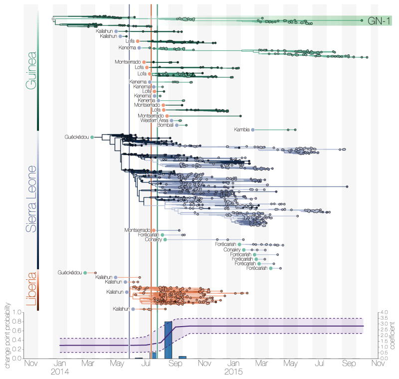
The first EBOV introduction from Guinea into another country that resulted in sustained transmission is estimated to have occurred in early April 2014 (Figure 2), when the virus spread to Kailahun District of Sierra Leone5, 6. This lineage was first detected in Kailahun at the end of May 2014, from where it spread across the region (Figures 4 & 3). From Kailahun EBOV spread extremely rapidly in May 2014 into several counties of Liberia (Lofa, Montserrado and Margibi)15 and Guinea (Conakry, back into Guéckédou)9, 11. The virus continued spreading westwards through Sierra Leone, and by July 2014 EBOV was present in the capital city, Freetown.
Figure 4. Transmission chains arising from independent international movements.
a) EBOV lineages by country (Guinea, green; Sierra Leone, blue; Liberia, red), tracked until the sampling date of their last known descendants. Circles at the roots of each subtree denote the country of origin for the introduced lineage. b) Estimates of the change point probability (primary Y-axis) and log coefficient (mean and credible interval; secondary Y-axis) for the Nat/Int factor. Vertical lines represent dates of border closures by the respective countries.
Figure 3. Dispersal of virus lineages over time.
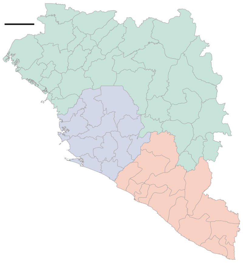
Virus dispersal between administrative regions estimated under the GLM phylogeography model (see Supplementary Methods). The arcs are between population centroids of each region, show directionality from thin end to thick end and are coloured in a scale denoting time from December 2013 in blue to October 2015 in yellow. Countries are coloured with Liberia in red, Guinea in green and Sierra Leone in blue.
By mid-September 2014 Liberia was reporting >500 new EVD cases per week, mostly driven by a large outbreak in Montserrado County, which encompasses the capital city, Monrovia. Sierra Leone reported >700 new cases per week by mid-November, with large outbreaks in Port Loko, Western Urban (Freetown) and Western Rural districts (Freetown suburbs). December 2014 brought the first signs that efforts to control the epidemic in Sierra Leone were effective as EVD incidence began dropping. By March 2015 the epidemic was largely under control in Liberia and eastern Guinea, although sustained transmission continued in the border area of western Guinea and western Sierra Leone. By the following month prevalence had declined such that only a handful of lineages persisted10, 12 (Figure 4).
The last EBOV genome resulting from a conventionally-acquired infection was collected and sequenced in October 2015 in Forécariah Prefecture (Guinea)10. After this, only sporadic cases of EVD were detected: in Montserrado (Liberia) in November 2015, Tonkolili (Sierra Leone) in January and February 2016, and Nzérékoré (Guinea) in March 2016. All these sporadic cases likely resulted from transmission from EVD survivors with established persistent infections12, 17, 18.
Factors associated with EBOV dispersal
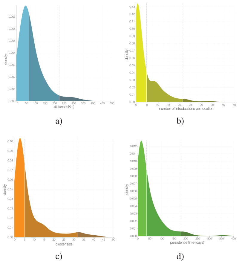
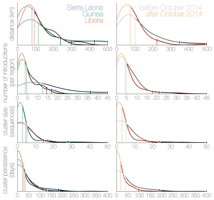
To determine the factors that influenced the spread of EBOV among administrative regions at the district (Sierra Leone), prefecture (Guinea) and county (Liberia) levels we used a phylogeographic generalized linear model (GLM)16. Of the 25 factors assessed (see Table 3 for a full list and description) five were included in the model with categorical support (Table 1). In summary, EBOV tends to disperse between geographically close regions (great circle distance: Bayes factor (BF) support for inclusion BF>50). Half of all virus dispersals occurred between locations <72 km apart and only 5% involved movement over 232 km (Figure 11a). Both origin and destination population sizes are very strongly (BF>50) positively correlated with viral dissemination, with a stronger effect for origin population size. The positive effect of population sizes combined with the inverse effect of geographic distance, implies that the epidemic’s spread followed a classic gravity-model dynamic. Gravity models, widely used in economic and geographic studies and a natural choice for modelling infectious disease transmission19–21, describe the movement of people between locations as a function of their population sizes and distance apart. Here we use viral genomes to provide empirical evidence that such a process drove viral dissemination during the EVD epidemic.
Table 3.
Predictors included in the time-homogenous GLM.
| Predictor type | Abbreviation | Predictor description |
|---|---|---|
| Geographic | Distances | Great circle distances between the locations’ population centroids, log-transformed, standardized |
| Administrative | Nat/Int | The relative preference of transitioning between locations in the same country over transitioning between locations in two different countries |
| Administrative | IntBoSh | The relative preference of transitioning between location pairs that are in different countries and share a border |
| Administrative | NatBoSh | The relative preference of transitioning between location pairs that are in the same country and share a border |
| Administrative | LibGinAsym | Between Liberia-Guinea asymmetry |
| Administrative | LibSLeAsym | Between Liberia-Sierra Leone asymmetry |
| Administrative | GinSLeAsym | Between Guinea-Sierra Leone asymmetry |
| Demographic | OrPop | Origin population size, log-transformed, standardized |
| Demographic | DestPop | Destination population size, log-transformed, standardized |
| Demographic | OrPopDens | Origin population density, log-transformed, standardized |
| Demographic | DestPopDens | Destination population density, log-transformed, standardized |
| Demographic | orTT100k | Estimated mean travel time in minutes to reach the nearest major settlement of at least 100,000 people at origin, log-transformed, standardized |
| Demographic | destinationTT100k | estimated mean travel time in minutes to reach the nearest major settlement of at least 100,000 people at destination, log-transformed, standardized |
| Demographic | OrGrEcon | Origin Gridded economic output, log-transformed, standardized |
| Demographic | DestGrEcon | Destination Gridded economic output, log-transformed, standardized |
| Cultural | IntLangShared | The relative preference of transitioning between location pairs that are in different countries and share at least one of 17 vernacular languages |
| Cultural | NatLangShared | The relative preference of transitioning between location pairs that are in the same country and share at least one of 17 vernacular languages |
| Climatic | OrTemp | Temperature annual mean at origin, log-transformed, standardized |
| Climatic | DestTemp | Temperature annual mean at destination, log-transformed, standardized |
| Climatic | OrTempSS | Index of temperature seasonality at origin, log-transformed, standardized |
| Climatic | DestTempSS | Index of temperature seasonality at destination, log-transformed, standardized |
| Climatic | OrPrecip | Precipitation annual mean at origin, log-transformed, standardized |
| Climatic | DestPrecip | Precipitation annual mean at destination, log-transformed, standardized |
| Climatic | OrPrecipSS | Index of precipitation seasonality at origin, log-transformed, standardized |
| Climatic | DestPrecipSS | Index of precipitation seasonality at destination, log-transformed, standardized |
Table 1.
Summary of phylogenetic generalized linear model results.
| Predictor1 | Description | Coefficient2 | 95% CI3 | Inclusion4 | BF5 |
|---|---|---|---|---|---|
| Nat/Int | National dispersal relative to international | 3.07 | 2.36, 3.77 | 1.0 | >50 |
| Distances | Great circle distances between the locations’ population centroids | −0.77 | −0.91, −0.63 | 1.0 | >50 |
| OrPop | Population size in the origin location | 1.36 | 0.86, 1.84 | 1.0 | >50 |
| DestPop | Population size in the destination location | 0.74 | 0.43, 1.06 | 1.0 | >50 |
| IntBoSh | Two locations share an international border | 3.39 | 2.42, 4.33 | 1.0 | >50 |
| originTmpss | Index of temperature seasonality at origin | −0.47 | −0.88, −0.11 | 0.1 | 3.79 |
Predictors included in the model with Bayes factor >3
Mean coefficient
95% highest posterior density credible interval (CI)
Probability that the predictor was included in the model
Bayes factor (BF)
Figure 11. The metapopulation structure of the epidemic.
a) Kernel density estimate (KDE) of distance for all inferred EBOV dispersals events: 50% occur over distances <72 km and <5% occur over distances >232 km. b) KDE of the number of independent EBOV introductions into each administrative region: 50% have fewer than 4.8 and <5% greater than 21.3. c) KDE of the mean size of sampled cases resulting from each introduction with at least 2 sampled cases: 50% < 5.3, 95% <32. d) KDE of the persistence of clusters in days (from time of introduction to time of the last sampled case): 50% < 36 days, 95% < 181 days.
In addition to geographical distance, we found a significant propensity for virus dispersal to occur within each country, relative to internationally (Nat/Int effect, BF>50), suggesting that country borders acted to curb the geographic spread of EBOV. When international dispersals do take place, they are more intense between administrative regions that are adjacent at an international border (IntBoSh, BF>50).
We tested whether sharing of any of 17 vernacular languages explains virus spread, as common languages might reflect cultural links including between non-contiguous or international regions, but found no evidence that such linguistic links were correlated with EBOV spread. A variety of other possible predictors of EBOV transmission, such as aspects of urbanization (economic output, population density, travel times to large settlements) and climatic effects, were not significantly associated with virus dispersal. However, these factors may have contributed to the size and longevity of transmission chains after introduction to a region (see below).
Finally, to investigate the potential of ‘real-time’ viral genome sequencing, we considered the degree to which the findings could have been obtained at the height of the epidemic, had sequences been available shortly after samples were taken (see Methods for details). For the factors associated with EBOV dispersal the results were extremely comparable with those for the full dataset with the same five factors being strongly supported and having similar effect sizes (Figure 5).
Figure 5. Inference of GLM predictors in a ‘real-time’ context.
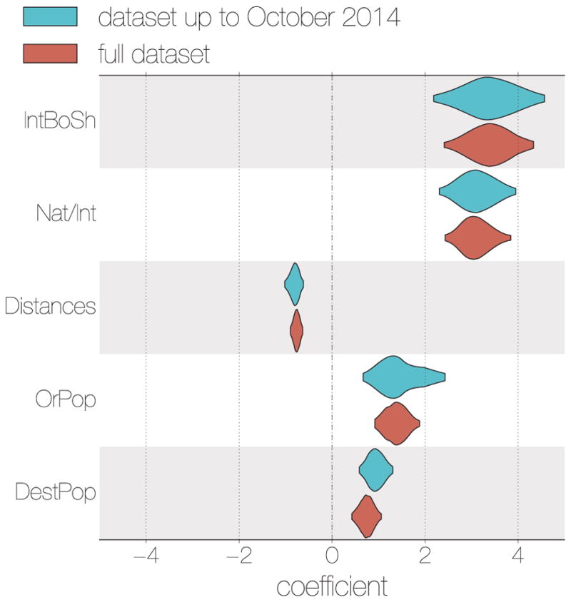
For the data set constructed from EBOV genome sequences derived from samples taken up until October 2014 (blue), the same 5 spatial EBOV movement predictors were given categorical support (inclusion probabilities = 1.0) as for the full data set (red). Likewise, the coefficients for these predictors are consistent in their sign and magnitude.
Factors associated with local EBOV proliferation
The analysis above identified predominantly geographical and administrative factors that predict the degree of importation risk, i.e. the likelihood that a viral lineage initiates at least one infection in a new region. However, the epidemiological consequences of each introduction—the size and duration of resulting transmission chains—may be affected by different factors. Thus we investigated which demographic, economic and climatic factors might predict cumulative case counts1 for each region (Bayesian GLM; see Methods) and found these were associated with factors related to urbanization (Table 2): primarily population sizes (PopSize, BF 29.6) and a significant inverse association with travel times to the nearest settlement with >50,000 inhabitants (tt50K, BF 32.4). These results confirm the common perception that, in contrast to previous EVD outbreaks, widespread transmission within urban regions in West Africa was a major contributing factor to the scale of the epidemic of the Makona variant.
Table 2.
Summary of generalized linear model results with case counts as the response variable.
| Predictor1 | Description | Coefficient2 | 95% CI3 | Inclusion4 | BF5 |
|---|---|---|---|---|---|
| TempSS | Temperature seasonality | −1.1 | −1.6, −0.5 | 0.83 | >50 |
| tt50K | Time to travel to a population centre of 50,000 people | −0.9 | −1.4, −0.4 | 0.62 | 32.4 |
| PopSize | Population size | 0.9 | 0.3, 1.6 | 0.60 | 29.6 |
| Precip | Precipitation | 0.8 | 0.2, 1.3 | 0.18 | 4.4 |
| tt100K | Time to travel to a population centre of 0.1 million people | −0.8 | −1.7, −0.1 | 0.16 | 3.8 |
Predictors included in the model with Bayes factor >3
Mean coefficient
95% highest posterior density credible interval (CI)
Probability that the predictor was included in the model
Bayes factor (BF)
As the epidemic in West Africa progressed there were fears that increased rainfall and humidity might prolong environmental persistence of EBOV particles, increasing the likelihood of transmission22. Although we found no evidence of an association between EBOV dispersal and any aspects of local climate, we find that regions with less seasonal variation in temperature, and more rainfall, tended to have larger EVD outbreaks (TempSS, BF >50 and Precip, BF 4.4 respectively).
Effect of international travel restrictions on EBOV dispersal
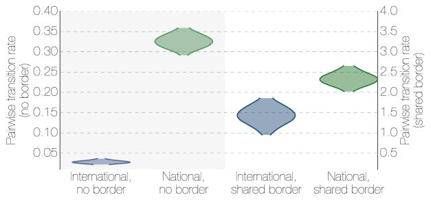
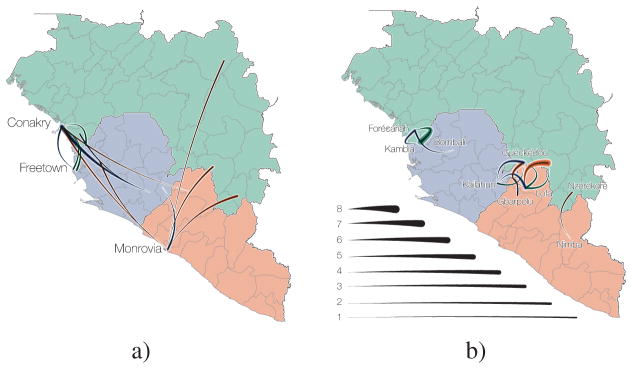
Porous borders between Liberia, Sierra Leone and Guinea may have allowed unimpeded EBOV spread during the 2013–2016 epidemic23–25. Our results indicate that international borders were associated with a decreased rate of transmission events compared to national borders (Figure 6), but that frequent international cross-border transmission events still occurred. These events were concentrated in Guéckédou Prefecture (Guinea), Kailahun District (Sierra Leone) and Lofa Country (Liberia) during the early phases of the epidemic (Figure 7a), and between Forécariah Prefecture (Guinea) and Kambia District (Sierra Leone) in the later stage (Figure 7b). These later EBOV movements significantly hindered efforts to interrupt the final chains of transmission in late 2015, with EBOV from such chains moving back and forth across this border10, 12, 26.
Figure 6. The effect of borders on EBOV migration rates between regions.
Posterior densities of the migration rates between locations that share a geographical border (left) and those that do not (right) for international migrations and national migrations. Where two regions share a border, national migrations are only marginally more frequent than international migrations showing that both types of borders are porous to short local movement. Where the two regions are not adjacent, international migrations are much rarer than national migrations.
Figure 7. Summarized epidemic international migration history.
All viral movement events between countries (Guinea, green; Sierra Leone, blue; Liberia, red) are shown split by whether they are between a) geographically distant regions or b) regions that share the international border. Curved lines indicate median (intermediate colour intensity), and 95% highest posterior density intervals (lightest and darkest colour intensities) for the number of migrations that are inferred to have taken place between countries.
Sierra Leone announced border closures on 11 June 2014, followed by Liberia on 27 July 2014, and Guinea on 9 August 2014, but little information is available about what these border closures actually entailed. Although we show that the relative contribution of international spread to overall viral migration was lower after country borders were closed (mean Nat/Int coefficient increasing from 1.15 to 2.83 between August and September 2014; 80.0% posterior support; (Figure 4b), it is difficult to ascertain whether the border closures themselves were responsible for the apparent reduction in cross-border transmissions, as opposed to concomitant control efforts or public information campaigns. However, even if border closures reduced international traffic, particularly over longer distances and between larger population centres, by the time Sierra Leone and Liberia closed their borders the epidemic had become firmly established in both countries (Figure 4).
Why did the epidemic not spread further?
A few EBOV exportations were documented from Guinea by road transport into Mali and Senegal27, 28 and by air from Liberia to Nigeria and USA29, 30. However, apart from these limited exceptions, the West African Ebola virus epidemic did not spread into the neighbouring regions of Côte d’Ivoire, Guinea-Bissau, Mali, and Senegal. By extending our GLM (the supported predictors and their estimated coefficients) to include these regions we were able to address whether they were spared EVD cases through good fortune, or because they were associated with an inherently lower risk of EBOV spread and transmission. We estimated the degree to which these, apparently EVD-free, regions had the potential to be exposed to viral introductions from affected regions (see Methods).
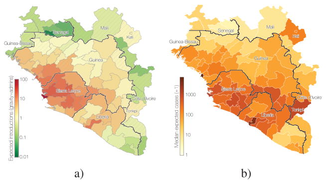
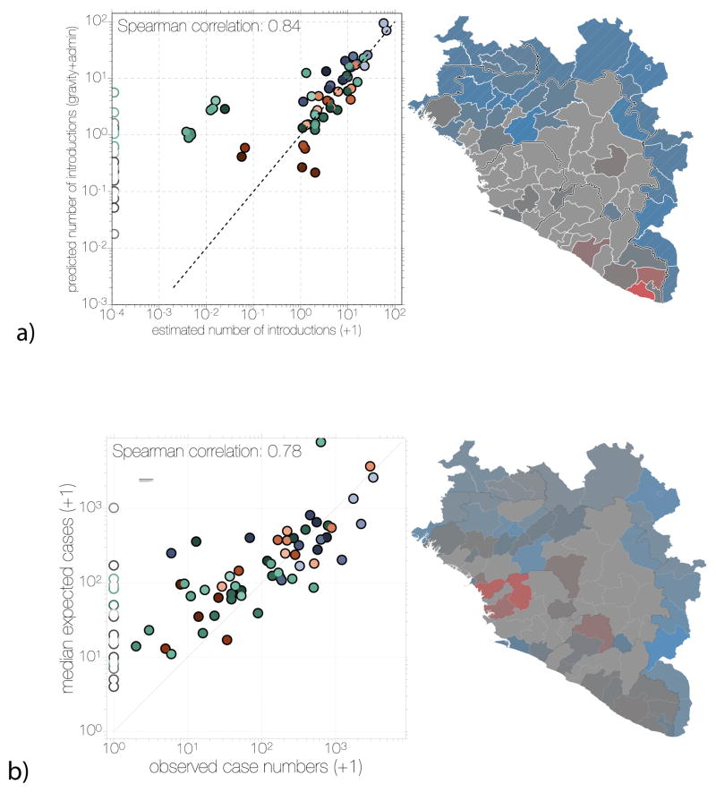
Overall, the contiguous regions in unaffected neighbouring countries were all predicted to have low numbers of EBOV introductions (Figures 8a and 9a) based on the phylogeographic history of the sampled cases. They were not, however, predicted to have particularly low levels of transmission if an outbreak had been seeded (Figures 8b and 9b). Thus, it is likely that some of these regions were at risk of becoming part of the EVD epidemic, but that their geographical distance from areas of active transmission and the attenuating effect of international borders prevented this from occurring. The Kati Cercle in Mali and Tonkpi Region in Côte d’Ivoire are to some extent exceptions to this general result, being more susceptible to EBOV introductions under the gravity model because of their large populations (1 million and 950,000, respectively), (Figure 8a) and predicted to have experienced many cases had EVD become established (Figure 8b).
Figure 8. Predicted destinations and consequences of viral dispersal.
a) Predicted number of EBOV imports into each of 63 regions in Guinea, Sierra Leone and Liberia (including 7 without recorded cases in Guinea) and the surrounding 18 regions of the neighbouring countries of Guinea-Bissau, Senegal, Mali and Côte d’Ivoire. The expected number of EBOV exports from locations in the phylogeographic tree and imports to any location were calculated based on the phylogeographic GLM model estimates and associated predictors that were extended to apparently EVD-free locations (see Methods). b) Predicted EVD cluster sizes from the generalized linear model fitted to case data.
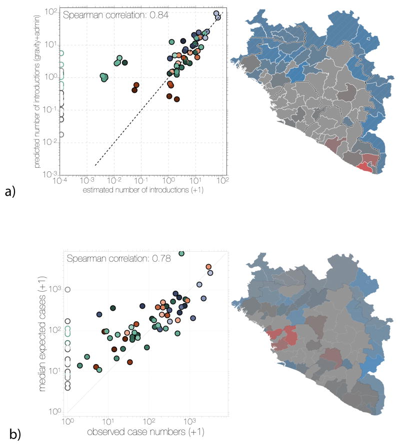
Figure 9. Comparison of predicted and observed numbers of introductions (a) and case numbers (b).
Scatter plots on the left of both panels show inferred introduction numbers (a) or observed case numbers (b), coloured by region as in Figure 4. Administrative regions not reporting any cases are indicated with empty circles on the scatter plot. Administrative regions in the map on the right side of both panels are coloured by the residuals (as observed/predicted) of the scatter plot. Regions are coloured grey where 0.5<observed/predicted<2.0 and transition into red or blue colours for overestimation or underestimation, respectively.
Metapopulation structure and dynamics of the EVD epidemic
After the initial establishment of transmission in Sierra Leone and Liberia, Guinea experienced repeated reintroductions of viral lineages from disparate transmission chains from both countries (Figure 4). Our analysis reveals that there were at least 21 (95% CI: 16 – 25) re-introductions into Guinea from April 2014 to February 2015. An early epidemic lineage was established around the Guinean capital, Conakry, and persisted for the duration of the epidemic (GN-1 in Figures 2 & 4). However, the continual ‘seeding’ of EBOV into Guinea without a clear peak in transmission suggests that elsewhere the virus may have been failing to maintain transmission. There were also numerous introductions into Sierra Leone over a similar time period (median: 9, 95% CI: 6 – 12) but the resulting transmission chains constituted a tiny proportion of the country’s EVD cases, with the bulk of transmission resulting from one early introduction (Figure 4a).
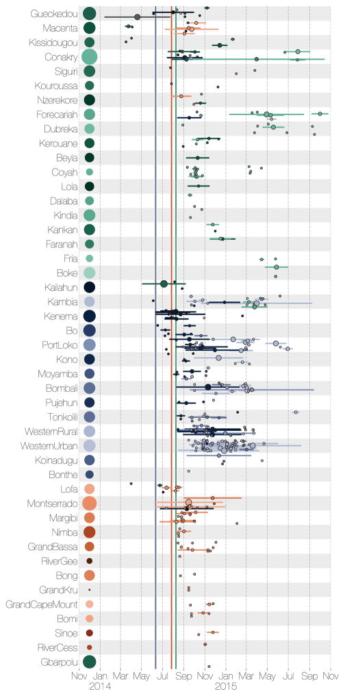
In all three countries, repeated seeding of administrative regions seems to have been a large factor in the longevity of the EVD epidemic (Figure 10). As such, regional case numbers were generally the result of multiple overlapping introduction events followed by within-region spread and occasional onward transmission to other regions. This suggests a metapopulation model in which the epidemic’s persistence was driven by introduction into novel contact networks rather than by mass-action susceptible-infectious-removed (SIR) dynamics31, 32. We found that, on average, EBOV migrates between administrative regions at a rate of 0.85 events per lineage per year (95% CI: 0.72, 0.97). Assuming a serial interval of 15.3 days33, this rate translates to a 3.6% chance (95% CI: 3.0%, 4.1%) that over the course of a single infection, the transmission chain moved between regions. Given the key role that virus dispersal played in sustaining the epidemic, the detection and isolation of these relatively low proportion of mobile cases may have a disproportionate effect on the control of an EVD epidemic.
Figure 10. Region specific introductions, cluster sizes and persistence.
Each row summarises independent introductions and the sizes (as numbers of sequences) of resulting outbreak clusters. Clusters are coloured by their inferred region of origin (colours same as Figure 4). The horizontal lines represent the persistence of each cluster from the time of introduction to the last sampled case (individual tips have persistence 0). The areas of the circles in the middle of the lines are proportional to the number of sequenced cases in the cluster. The areas of the circles next to the labels on the left represent the population sizes of each administrative region. Vertical lines within each cell indicate the dates of declared border closures by each of the three countries: 11 June 2014 in Sierra Leone (blue), 27 July 2014 in Liberia (red), and 09 August 2014 in Guinea (green).
From our spatial phylogenetic model we conclude that many regions experienced numerous independent EBOV introductions (Figure 11b). However, these introductions gave rise to clusters of cases that were generally small (a mean cluster size of 4.3 and only 5% larger than 17 in our sample; Figure 11c) and of limited duration (a mean persistence time of 41.3 days with only 5% greater than 181 days; Figure 11d). Here, we define a ‘cluster’ as a group of sequenced cases in a region that derive from a single introduction event and define ‘persistence’ as the time between the introduction event and the last sampled case in the cluster. These definitions are conservative regarding sampling intensity as we expect additional samples would have split clusters apart rather than join them. Furthermore, introductions that were not detected will be disproportionately smaller, and so the cluster size estimate will be biased upwards. Segregating these observations by country (Figure 12a) shows that districts of Sierra Leone had more introductions and Guinea generally had smaller clusters but persistence was similar between the three countries. Considering only introductions that occurred before October 2014 to those that occurred after, the number of introductions per location was comparable whereas those that occurred early generally resulted in larger and more persistent clusters (Figure 12b).
Figure 12.
Kernel density estimates for inferred epidemiological statistics (from top to bottom): distance travelled (distance between population centroids, in kilometres), number of introductions that each location experienced, cluster size (number of sequences collected in a location as a result of a single introduction), cluster persistence (days from the common ancestor of a cluster to its last descendent, single tips have persistence of 0). Left hand side tracks these statistics for Sierra Leone (blue), Liberia (red) and Guinea (green), whilst the right hand side compares the statistics for before October 2014 (grey) and after (orange). Points with vertical lines connected to the x axis indicate the 50% and 95% quantiles of the parameter density estimates. Within Sierra Leone, Liberia and Guinea, 50% of all migrations occurred over distances of around 100km and persisted for around 25 days. Exceptions were Sierra Leone which experienced more introductions per location (around 12) than Guinea and Liberia (around 4) and Guinea, where migrations tended to occur over larger distances due to the size of the country and whose cluster sizes following introductions tended to be lower (3 sequences versus Liberia and Sierra Leone with 5 sequences each). Between the first (grey) and second (orange) years of the epidemic there were considerable reductions in cluster persistence, cluster sizes and distances travelled by viruses, whilst dispersal intensity remained largely the same.
Thus, with 5.8% sampling, we arrive at a conservative estimate of approximately 75 regional cases per introduction event. Although larger population centres, in particular capital cities, generally experienced more introductions (Figure 13a), the cluster sizes are less strongly associated with population size (Figure 13b), further highlighting the role of virus movement into urban areas as major factor for the high case loads in large population centres. Frequent cluster extinction, despite a small fraction of individuals being infected, suggests that individual outbreaks were constrained by the degree of connectedness among contact networks. Thus, it appears that the West African EVD epidemic was sustained by frequent seeding that resulted in numerous small local clusters of cases, some of which went on to seed further local clusters.
Figure 13. Relationship of cluster size, introductions and persistence to population size.
a) The mean number of introductions into each location against (log) population sizes. The Western Area (in Sierra Leone) received the most introductions, whilst Conakry (in Guinea) and Montserrado (in Liberia) were closer to the average. The association between population sizes and number of introductions was not very strong (R2 = 0.28, pearson correlation = 0.54, Spearman correlation = 0.57). b) The mean cluster size for each location plotted against (log) population sizes. The association here is weaker (R2 = 0.11, pearson correlation = 0.35, Spearman correlation = 0.57). c) The mean persistence times (per cluster, in days) against population sizes. A similarly weak association is observed (R2 = 0.12, pearson correlation = 0.37, Spearman correlation = 0.36). All computations based on a sample of 10,000 trees from the posterior distribution.
Viral genomics as a tool for outbreak response
The 2013–2016 EVD epidemic in West Africa has unfortunately become a costly lesson in addressing an infectious disease outbreak in the absence of preparedness of both the exposed population and the international community. Our work demonstrates the value of pathogen genome sequencing in a public healthcare emergency and the value of timely pre-publication data sharing to identify the origins of imported disease case clusters, to track pathogen transmission as the epidemic progresses, and to follow up on individual cases as the epidemic subsides.
It is inevitable that as sequencing costs decrease, accuracy increases, and sequencing instruments become more portable, real-time viral surveillance and molecular epidemiology will be routinely deployed on the front lines of infectious disease outbreaks10, 12, 14, 34–36. Although we have shown here that the broad pattern of EBOV spatial movement was discernible from virus genomes derived from samples collected only up until October 2014, there was a notable hiatus in sequencing at this time35 and the genomes in the present data set from that time were sequenced retrospectively from archived material. The West African EVD epidemic has demonstrated that a steady sequencing pace34–36, local sequencing capacity10, 12, 14 and rapid dissemination of data7 are key ingredients in generating actionable sequence data from an infectious disease outbreak. However, as viral genome sequencing is scaled up and approaches the time-scale of viral evolution, the analysis techniques will increasingly represent the bottleneck for timely communication of information for outbreak response.
The analysis of the comprehensive EBOV genome set collected during the 2013–2016 EVD epidemic, including the findings presented here and in other studies7, 9, 11–15, 37, 38 provides a framework for predicting the behaviour of future disease outbreaks caused by EBOV, other filoviruses, and perhaps other human pathogens. However, many open questions remain about the biology of EBOV. As sustained human-to-human transmission waned, West Africa experienced several instances of recrudescent transmission, often in regions that had not seen cases for many months as a result of persistent sub-clinical infections17, 18, 39. Although, in hindsight, such sequelae were not entirely unexpected40, the magnitude of the 2013–2016 epidemic has put the region at ongoing risk of sporadic EVD re-emergence. Similarly, the nature of the reservoir of EBOV, and its geographic distribution, remain as fundamental gaps in our knowledge. Resolving these questions is critical to predicting the risk of zoonotic transmission and hence of future EVD outbreaks.
Methods
Sequence data
We compiled a data set of 1,610 publicly available full Ebola virus (EBOV) genomes sampled between 17 March 2014 and 24 October 2015 (see https://github/ebov/space-time/data/ for full list and metadata). The number of sequences and the proportion of cases sequenced varies with country; our data set contains 209 sequences from Liberia (3.8% of known and suspected cases), 982 from Sierra Leone (8.0%) and 368 from Guinea (9.2%) (Supplementary Table 1). Most (N=1,100) genomes are of high quality, with ambiguous sites and gaps comprising less than 1% of total alignment length, followed by sequences with between 1% and 2% of sites comprised of ambiguous bases or gaps (N=266), 98 sequences with 2–5%, 120 sequences with 5–10% and 26 sequences with more than 10% of sites that are ambiguous or are gaps. Sequences known to be associated with sexual transmission or latent infections were excluded, as these viruses often exhibit anomalous molecular clock signals17, 18. Sequences were aligned using MAFFT41 and edited manually. The alignment was partitioned into coding regions and non-coding intergenic regions with a final alignment length of 18,992 nucleotides (available from https://github/ebov/space-time/data/).
Masking putative ADAR edited sites
As noticed by Tong et al.38, Park et al.13 and other studies, some EBOV isolates contain clusters of T-to-C mutations within relatively short stretches of the genome. Interferon-inducible adenosine deaminases acting on RNA (ADAR) are known to induce adenosine to inosine hypermutations in double-stranded RNA42. ADARs have been suggested to act on RNAs from numerous groups of viruses43. When negative sense single stranded RNA virus genomes are edited by ADARs, A-to-G hypermutations seem to preferentially occur on the negative strand, which results in U/T-to-C mutations on the positive strand44–46. Multiple T-to-C mutations are introduced simultaneously via ADAR-mediated RNA editing which would interfere with molecular clock estimates and, by extension, the tree topology. We thus designate four or more T-to-C mutations within 300 nucleotides of each other as a putative hypermutation tract, whenever there is evidence that all T-to-C mutations within such stretches were introduced at the same time, i.e. every T-to-C mutation in a stretch occurred on a single branch. We detect a total of 15 hypermutation patterns with up to 13 T-to-C mutations within 35 to 145 nucleotides. Of these patterns, 11 are unique to a single genome and 4 are shared across multiple isolates, suggesting that occasionally viruses survive hypermutation are transmitted47. Putative tracts of T-to-C hypermutation almost exclusively occur within non-coding intergenic regions, where their effects on viral fitness are presumably minimal. In each case we mask out these sites as ambiguous nucleotides but leave the first T-to-C mutation unmasked to provide phylogenetic information on the relatedness of these sequences.
Phylogenetic inference
Molecular evolution was modelled according to a HKY+Γ448, 49 substitution model independently across four partitions (codon positions 1, 2, 3 and non-coding intergenic regions). Site-specific rates were scaled by relative rates in the four partitions. Evolutionary rates were allowed to vary across the tree according to a relaxed molecular clock that draws branch-specific rates from a log-normal distribution50. A non-parametric coalescent ‘Skygrid’ model was used to act as a prior density across trees51. The overall evolutionary rate was given an uninformative continuous-time Markov chain (CTMC) reference prior52, while the rate multipliers for each partition were given an uninformative uniform prior over their bounds. All other priors used to infer the phylogenetic tree were left at their default values. BEAST XML files are available from https://github/ebov/space-time/data/. We ran an additional analysis with a subset of data (787 sequences collected up to November 2014 — the peak of case numbers in Sierra Leone) to test the robustness of inference if they had been performed mid-epidemic.
Geographic history reconstruction
The level of administrative regions within each country was chosen so that population sizes between regions are comparable. For each country the appropriate administrative regions were: prefecture for Guinea (administrative subdivision level 2), county for Liberia (level 1) and district for Sierra Leone (level 2). We refer to them as regions (63 in total but only 56 are recorded to have had EVD cases) and each sequence, where available, was assigned the region where the patient was recorded to have been infected as a discrete trait. When the region within a country was unknown (N=223), we inferred the sequence location as a latent variable with equal prior probability over all available regions within that country. Most of the sequences with unknown regional origins were from Sierra Leone (N=151), followed by Liberia (N=69) and Guinea (N=3). In the absence of any geographic information (N=2) we inferred both the country and the region of a sequence.
We deploy an asymmetric continuous-time Markov chain (CTMC)53, 54 matrix to infer instantaneous transitions between regions. For 56 regions with recorded EVD cases, a total of 3080 independent transition rates would be challenging to infer from one realisation of the process, even when reduced to a sparse migration matrix using stochastic search variable selection (SSVS)53.
Thus, to infer the spatial phylogenetic diffusion history between the K = 56 locations, we adopt a sparse generalized linear model (GLM) formulation of continuous-time Markov chain (CTMC) diffusion16. This model parameterizes the instantaneous movement rate Λij from location i to location j as a log-linear function of P potential predictors Xij = (xij1, …, xijP)′ with unknown coefficients β = (β1, …, βP)′ and diagonal matrix δ with entries (δ1, …, δP). These latter unknown indicators δp ∈ {0, 1} determine predictor p’s inclusion in or exclusion from the model. We generalize this formulation here to include two-way random effects that allow for location origin- and destination-specific variability. Our two-way random effects GLM becomes
| (1) |
where ε = (ε1, …, εK) are the location-specific effects. These random effects account for unexplained variability in the diffusion process that may otherwise lead to spurious inclusion of predictors.
We follow16 in specifying that a priori all βp are independent and normally distributed with mean 0 and a relatively large variance of 4 and in assigning independent Bernoulli prior probability distributions on δp.
Let q be the inclusion probability and w be the probability of no predictors being included. Then, using the distribution function of a binomial random variable q = 1 − w1/P, where P is the number of predictors, as before. We use a small success probability on each predictor’s inclusion that reflects a 50% prior probability (w) on no predictors being included.
In our main analysis, we consider 25 individual predictors that can be classified as geographic, administrative, demographic, cultural and climatic covariates of spatial spread (Table 3). Where measures are region-specific (rather than pairwise region measures), we specify both an origin and destination predictor. We also tested for sampling bias by including an additional origin and destination predictor based on the residuals for the regression of sample size against case count (cfr. Figure 1b), but these predictors did not receive any support (data not shown).
To draw posterior inference, we follow16 in integrating β and δ, and further employ a random-walk Metropolis transition kernel on ε and sample σ2 directly from its full conditional distribution using Gibbs sampling.
To obtain a joint posterior estimate from this joint genetic and phylogeographic model, an MCMC chain was run in BEAST 1.8.455 for 100 million states, sampling every 10 000 states. The first 1000 samples in each chain were removed as burnin, and the remaining 9 000 samples used to estimate a maximum clade credibility tree and to estimate posterior densities for individual parameters. A second independent run of 100 million states was performed to check convergence of the first.
To consider the feasibility of ‘real-time’ inference from virus genome data from the height of the EVD epidemic we took only those sequences derived from samples taken up until the end of October 2014 (N = 787). We undertook the same joint phylogenetic and spatial GLM analysis as for the full data set including the same set of 25 predictors. We ran this analysis for 200 million states, sampling every 20,000 states and removing the first 10% of samples.
To obtain realisations of the phylogenetic CTMC process, including both transitions (Markov jumps) between states and waiting times (Markov rewards) within states, we employ posterior inference of the complete Markov jump history through time16, 56. In addition to transitions ‘within’ the phylogeny, we also estimate the expected number of transitions ‘from’ origin location i in the phylogeographic tree to arbitrary ‘destination’ location j as follows:
| (2) |
where τi is the waiting time (or Markov reward) in ‘origin’ state i throughout the phylogeny, μ is the overall rate scalar of the location transition process, πi is the equilibrium frequency of ‘origin’ state i, and c is the normalising constant applied to the CTMC rate matrices in BEAST. To obtain the expected number of transitions to a particular destination location from any phylogeographic location (integrating over all possible locations across the phylogeny), we sum over all 56 origin locations included in the analysis. We note that the destination location can also be a location that was not included in the analysis because we only need to consider destination j in the instantaneous movement rates Λij; since the log of these rates are parameterized as a log linear function of the predictors, we can obtain these rates through the coefficient estimates from the analysis and the predictors extended to include these additional locations. Specifically, we use this to predict introductions in regions in Guinea, for which no cases were reported (n = 7) and for regions in neighbouring countries along the borders with Guinea or Liberia that remained disease free (n = 18). To obtain such estimates under different predictors or predictor combinations, we perform a specific analysis under the GLM model including only the relevant predictors or predictor combinations without the two-way random effects. For computational expedience, we performed these analyses, as well as the time-inhomogeneous analyses below, by conditioning on a set of 1,000 trees from the posterior distribution of the main phylogenetic analysis16. We summarize mean posterior estimates for the transition expectations based on the samples obtained by our MCMC analysis; we note that also the value of c is sample-specific.
Time-dependent spatial diffusion
To consider time-inhomogeneity in the spatial diffusion process, we start by borrowing epoch modelling concepts from Bielejec et al. (2014)57. The epoch GLM parameterizes the instantaneous movement rate Λijt from state i to state j within epoch t as a log-linear function of P epoch-specific predictors Xijt = (xijt1, …, xijtP)′ with constant-through-time, unknown coefficients β. We generalize this model to incorporate time-varying contribution of the predictors through time-varying coefficients β(t) using a series of change-point processes. Specifically, the time-varying epoch GLM models
| (3) |
where βB = (βB1, …, βBP)′ are the unknown coefficients before the change-points, βA = (βA1, …, βAP)′ are the unknown coefficients after the change-points, diagonal matrix ϕ(t) has entries (1t>t1(t), …, 1t>tP(t)), 1(·)(t) is the indicator function and T = (t1, …, tP) are the unknown change-point times. In this general form, the contribution of predictor p before its change-point time tp is βBp and its contribution after is βAp for p = 1, …, P. Fixing tp to be less than the time of the first epoch or greater than the time of the last epoch results in a time-invariant coefficient for that predictor.
Similar to the constant-through-time GLM, we specify that a priori all βBp and βAp are independent and normally distributed with mean 0 and a relatively large variance of 4. Under the prior, each tp is equally likely to lie before any epoch.
We employ random-walk Metropolis transition kernels on βB, βA and T.
In a first epoch GLM analysis, we keep the five predictors that are convincingly supported by the time-homogeneous analysis included in the model and estimate an independent change-point tp for their associated effect sizes: distance (tdis), within country effect (twco), shared international border (tsib) and origin and destination population size (tpopo and tpopd) change-points. To quantify the evidence in favour of each change-point, we calculate Bayes factor support based on the prior and posterior odds that tp is less than the time of the first epoch or greater than the time of the last epoch. Because we find only very strong support for a change-point in the within country effect, we subsequently estimate the effect sizes before and after twco, keeping the remaining four predictors homogeneous through time.
Within-location generalized linear models
Ebola virus disease (EVD) case numbers are reported by the WHO for every country division (region) at the appropriate administrative level, split by epidemiological week. For every region and for each epidemiological week four numbers are reported: new cases in the patient and situation report databases as well as whether the new cases are confirmed or probable. At the height of the epidemic many cases went unconfirmed, even though they were likely to have been genuine EVD. As such, we treat probable EVD cases in WHO reports as confirmed and combine them with lab-confirmed EVD case numbers. Following this we take the higher combined case number of situation report and patient databases. The latest situation report in our data goes up to the epidemiological week spanning 8 to 14 February 2016, with all case numbers being downloaded on 22 February 2016. There are apparent discrepancies between cumulative case numbers reported for each country over the entire epidemic and case numbers reported per administrative division over time, such that our estimate for the final size of the epidemic, based on case numbers over time reported by the WHO, is on the order of 22 000 confirmed and suspected cases of EVD compared to the official estimate of around 28 000 cases across the entire epidemic. This likely arose because case numbers are easier to track at the country level, but become more difficult to narrow down to administrative subdivision level, especially over time (only 86% of the genome sequence have known location of infection).
We studied the association between disease case counts using generalized linear models in a very similar fashion to the framework presented above. A list of the location-level predictors we used for these analyses can be found in Table 3. We also employed SSVS as described above, in order to compute Bayes factors (BF) for each predictor. In keeping with the genetic GLM analyses, we also set the prior inclusion probabilities such that there was a 50% probability of no predictors being included.
where r is the over-dispersion parameter, δi are the indicators as before. Prior distributions on model parameters for these analyses were the same as those used for the genetic analyses whenever possible. We then employed this model to predict how many cases the locations which reported zero EVD cases would have gathered, that is, the potential size of the epidemic in each location.
Computational details
To fit the models described above we took advantage of the routines already built in BEAST (https://github.com/beast-dev/beast-mcmc) but in a non-phylogenetic setting. Once again, posterior distributions for the parameters were explored using Markov chain Monte Carlo (MCMC). We ran each chain for 50 million iterations and discarded at least 10% of the samples as burn-in. Convergence was checked by visual inspection of the chains and checking that all parameters had effective sample sizes (ESS) greater than 200. We ran multiple chains to ensure results were consistent. To make predictions, we used 50,000 Monte Carlo samples from the posterior distribution of coefficients and the overdispersion parameter (r) to simulate case counts for all locations with zero recorded EVD cases.
Data availability
All collated data, genetic sequence alignments, phylogenetic trees, analysis scripts, and analysis output are available at https://github.com/ebov/space-time) and http://dx.doi.org/10.7488/ds/1711. Individual virus genetic sequences are published in earlier works and are available from NCBI Genbank.
Supplementary Material
Acknowledgments
The authors acknowledge support from: European Union Seventh Framework 278433-PREDEMICS (P.L., A.R.) and ERC 260864 (P.L., A.R., M.A.S.) European Union Horizon 2020 643476-COMPARE (M.P.G.K., A.R.), 634650-VIROGENESIS (P.L., M.P.G.K.), 666100-EVIDENT and European Commission IFS/2011/272-372, EMLab (S.G.), National Institutes of Health R01 AI107034, R01 AI117011 and R01 HG006139 and National Science Foundation IIS 1251151 and DMS 1264153 (M.A.S.), NIH AI081982, AI082119, AI082805 AI088843, AI104216, AI104621, AI115754, HSN272200900049C, HHSN272201400048C (R.F.G.), National Health & Medical Research Council (Australia) (E.C.H.). The Research Foundation - Flanders G0D5117N (G.B., P.L.), Work in Liberia was funded by the Defense Threat Reduction Agency, the Global Emerging Infections System, and the _targeted Acquisition of Reference Materials Augmenting Capabilities (TARMAC) Initiative agencies from the U.S. Department of Defense (G.P.), Bill and Melinda Gates Foundation OPP1106427, 1032350, OPP1134076, Wellcome Trust 106866/Z/15/Z, Clinton Health Access Initiative (A.J.T.), National Institute for Health Research Health Protection Research Unit in Emerging and Zoonotic Infections (J.A.H.), Key Research and Development Program from the Ministry of Science and Technology of China 2016YFC1200800 (D.L.), National Natural Science Foundation of China 81590760 and 81321063 (G.F.G.), Mahan Post-doctoral fellowship Fred Hutchinson Cancer Research Center (G.D.), National Institute of Allergy and Infectious Disease U19AI110818, 5R01AI114855-03, United States Agency for International Development OAA-G-15-00001 and the Bill and Melinda Gates Foundation OPP1123407-(P.C.S.), NIH 1U01HG007480-01 and the World Bank ACE019 (C.T.H.), PEW Biomedical Scholarship, NIH UL1TR001114, and NIAID contract HHSN272201400048C (K.G.A.)
J.H.K., an employee of Tunnell Government Services, Inc., is a subcontractor under Battelle Memorial Institute’s prime contract with the NIAID (contract HHSN272200700016I).
Colour-blind-friendly colour palettes designed by Cynthia Brewer, Pennsylvania State University (http://colorbrewer2.org). Matplotlib (http://matplotlib.org) was used extensively throughout this article for data visualisation. We gratefully acknowledge support from NVIDIA Corporation with the donation of parallel computing resources used for this research.
Finally, we would like to recognize the contributions made by our colleagues who tragically died from Ebola virus disease whilst fighting the epidemic. In particular, we honour the memory of Dr. Sheik Humarr Khan and Nurse Mbalu Fonnie, whose careers were dedicated to viral hemorrhagic fever research.
Footnotes
Supplementary Information is available in the online version of the paper.
Author Contributions G.D., L.M.C., T.B., C.F., M.A.S., P.L., and A.R. designed the study. G.D., L.M.C., T.B., A.J.T., G.B., P.L., and A.R. performed the analysis. G.D., T.B., M.A.S, P.L., and A.R. wrote the manuscript. L.M.C., A.J.T., G.B., N.R.F., J.T.L., M.C., S.F.S., K.G.A., M.W.C., R.F.G., I.G., E.C.H., P.K., M.P.G.K., J.H.K., S.T.N., G.P., O.G.P., P.C.S., and U.S. edited the manuscript. Other authors were critical to the coordination, collection, processing of virus samples or sequencing and bioinformatics of virus genomes. All authors read and approved the contents of the manuscript.
The authors declare no competing financial interests.
Readers are welcome to comment on the online version of the paper.
References
- 1.World Health Organization. Ebola situation report - 10 june 2016. 2016 URL http://apps.who.int/iris/bitstream/10665/208883/1/ebolasitrep_10Jun2016_eng.pdf.
- 2.Kuhn JH, et al. Nomenclature- and database-compatible names for the two ebola virus variants that emerged in guinea and the democratic republic of the congo in 2014. Viruses. 2014;6:4760–4799. doi: 10.3390/v6114760. URL http://dx.doi.org/10.3390/v6114760. [DOI] [PMC free article] [PubMed] [Google Scholar]
- 3.Baize S, et al. Emergence of zaire ebola virus disease in guinea. The New England Journal of Medicine. 2014;371:1418–1425. doi: 10.1056/NEJMoa1404505. URL http://dx.doi.org/10.1056/NEJMoa1404505. [DOI] [PubMed] [Google Scholar]
- 4.World Health Organization Regional Office for Africa. Ebola virus disease, west africa (situation as of 25 april 2014) 2014 URL http://www.afro.who.int/en/clusters-a-programmes/dpc/epidemic-a-pandemic-alert-and-response/4121-ebola-virus-disease-west-africa-25-april-2014.html.
- 5.Goba A, et al. An outbreak of ebola virus disease in the lassa fever zone. The Journal of infectious diseases. 2016 doi: 10.1093/infdis/jiw239. URL http://dx.doi.org/10.1093/infdis/jiw239. [DOI] [PMC free article] [PubMed]
- 6.Sack K, Fink S, Belluck P, Nossiter A, Berehulak D. How ebola roared back. 2014 URL http://nyti.ms/1wwG5VX.
- 7.Gire SK, et al. Genomic surveillance elucidates ebola virus origin and transmission during the 2014 outbreak. Science. 2014;345:1369–1372. doi: 10.1126/science.1259657. URL http://www.sciencemag.org/content/345/6202/1369. [DOI] [PMC free article] [PubMed] [Google Scholar]
- 8.Dudas G, Rambaut A. Phylogenetic analysis of guinea 2014 ebov ebolavirus outbreak. PLoS Currents. 2014;6 doi: 10.1371/currents.outbreaks.84eefe5ce43ec9dc0bf0670f7b8b417d. URL http://www.ncbi.nlm.nih.gov/pmc/articles/PMC4024086/ [DOI] [PMC free article] [PubMed] [Google Scholar]
- 9.Carroll MW, et al. Temporal and spatial analysis of the 2014–2015 ebola virus outbreak in west africa. Nature. 2015;524:97–101. doi: 10.1038/nature14594. URL http://www.nature.com/nature/journal/v524/n7563/full/nature14594.html. [DOI] [PMC free article] [PubMed] [Google Scholar]
- 10.Quick J, et al. Real-time, portable genome sequencing for ebola surveillance. Nature. 2016;530:228–232. doi: 10.1038/nature16996. URL http://www.nature.com/nature/journal/v530/n7589/full/nature16996.html. [DOI] [PMC free article] [PubMed] [Google Scholar]
- 11.Simon-Loriere E, et al. Distinct lineages of ebola virus in guinea during the 2014 west african epidemic. Nature. 2015;524:102–104. doi: 10.1038/nature14612. URL http://www.nature.com/nature/journal/v524/n7563/full/nature14612.html. [DOI] [PMC free article] [PubMed] [Google Scholar]
- 12.Arias A, et al. Rapid outbreak sequencing of ebola virus in sierra leone identifies transmission chains linked to sporadic cases. Virus Evolution. 2016;2:vew016. doi: 10.1093/ve/vew016. URL http://dx.doi.org/10.1093/ve/vew016. [DOI] [PMC free article] [PubMed] [Google Scholar]
- 13.Park DJ, et al. Ebola virus epidemiology, transmission, and evolution during seven months in sierra leone. Cell. 2015;161:1516–1526. doi: 10.1016/j.cell.2015.06.007. URL http://www.sciencedirect.com/science/article/pii/S009286741500690X. [DOI] [PMC free article] [PubMed] [Google Scholar]
- 14.Kugelman JR, et al. Monitoring of ebola virus makona evolution through establishment of advanced genomic capability in liberia. Emerging infectious diseases. 2015;21:1135–1143. doi: 10.3201/eid2107.150522. URL http://dx.doi.org/10.3201/eid2107.150522. [DOI] [PMC free article] [PubMed] [Google Scholar]
- 15.Ladner JT, et al. Evolution and spread of ebola virus in liberia, 2014– 2015. Cell host and microbe. 2015;18:659–669. doi: 10.1016/j.chom.2015.11.008. URL http://www.sciencedirect.com/science/article/pii/S193131281500462X. [DOI] [PMC free article] [PubMed] [Google Scholar]
- 16.Lemey P, et al. Unifying Viral Genetics and Human Transportation Data to Predict the Global Transmission Dynamics of Human Influenza H3n2. PLoS Pathog. 2014;10:e1003932. doi: 10.1371/journal.ppat.1003932. URL http://journals.plos.org/plospathogens/article?id=10.1371/journal.ppat.1003932. [DOI] [PMC free article] [PubMed] [Google Scholar]
- 17.Blackley DJ, et al. Reduced evolutionary rate in reemerged ebola virus transmission chains. Science advances. 2016;2:e1600378. doi: 10.1126/sciadv.1600378. URL http://dx.doi.org/10.1126/sciadv.1600378. [DOI] [PMC free article] [PubMed] [Google Scholar]
- 18.Mate SE, et al. Molecular evidence of sexual transmission of ebola virus. The New England Journal of Medicine. 2015;373:2448–2454. doi: 10.1056/NEJMoa1509773. URL http://dx.doi.org/10.1056/NEJMoa1509773. [DOI] [PMC free article] [PubMed] [Google Scholar]
- 19.Viboud C, et al. Synchrony, waves, and spatial hierarchies in the spread of influenza. Science. 2006;312:447–451. doi: 10.1126/science.1125237. URL http://dx.doi.org/10.1126/science.1125237. [DOI] [PubMed] [Google Scholar]
- 20.Truscott J, Ferguson NM. Evaluating the adequacy of gravity models as a description of human mobility for epidemic modelling. PLoS computational biology. 2012;8:e1002699. doi: 10.1371/journal.pcbi.1002699. URL http://www.ploscompbiol.org/article/info:doi/10.1371/journal.pcbi.1002699;jsessionid=CF06777280C342A9BF39AD70509903EC. [DOI] [PMC free article] [PubMed] [Google Scholar]
- 21.Yang W, et al. Transmission network of the 2014–2015 ebola epidemic in sierra leone. Journal of the Royal Society, Interface / the Royal Society. 2015;12:20150536. doi: 10.1098/rsif.2015.0536. URL http://rsif.royalsocietypublishing.org/content/12/112/20150536. [DOI] [PMC free article] [PubMed] [Google Scholar]
- 22.Fischer R, et al. Ebola virus stability on surfaces and in fluids in simulated outbreak environments. Emerging infectious diseases. 2015;21:1243–1246. doi: 10.3201/eid2107.150253. URL http://dx.doi.org/10.3201/eid2107.150253. [DOI] [PMC free article] [PubMed] [Google Scholar]
- 23.Bausch DG, Schwarz L. Outbreak of ebola virus disease in guinea: Where ecology meets economy. PLoS neglected tropical diseases. 2014;8:e3056. doi: 10.1371/journal.pntd.0003056. URL http://dx.doi.org/10.1371/journal.pntd.0003056. [DOI] [PMC free article] [PubMed] [Google Scholar]
- 24.Chan M. Ebola virus disease in west africa–no early end to the outbreak. The New England Journal of Medicine. 2014;371:1183–1185. doi: 10.1056/NEJMp1409859. URL http://dx.doi.org/10.1056/NEJMp1409859. [DOI] [PubMed] [Google Scholar]
- 25.Wesolowski A, et al. Commentary: containing the ebola outbreak - the potential and challenge of mobile network data. PLoS currents. 2014;6 doi: 10.1371/currents.outbreaks.0177e7fcf52217b8b634376e2f3efc5e. URL http://dx.doi.org/10.1371/currents.outbreaks.0177e7fcf52217b8b634376e2f3efc5e. [DOI] [PMC free article] [PubMed] [Google Scholar]
- 26.Goodfellow I, Reusken C, Koopmans M. Laboratory support during and after the ebola virus endgame: towards a sustained laboratory infrastructure. Euro surveillance. 2015;20 doi: 10.2807/1560-7917.es2015.20.12.21074. URL http://www.ncbi.nlm.nih.gov/pubmed/25846492. [DOI] [PubMed] [Google Scholar]
- 27.World Health Organization. Ebola response roadmap situation report update - november 2014. 2014 URL http://apps.who.int/iris/bitstream/10665/141468/1/roadmapsitrep_12Nov2014_eng.pdf.
- 28.Folarin OA, et al. Ebola virus epidemiology and evolution in nigeria. The Journal of infectious diseases. 2016 doi: 10.1093/infdis/jiw190. URL http://dx.doi.org/10.1093/infdis/jiw190. [DOI] [PMC free article] [PubMed]
- 29.Abdoulaye B, et al. Experience on the management of the first imported ebola virus disease case in senegal. The Pan African medical journal. 2015;22(Suppl 1):6. doi: 10.11694/pamj.supp.2015.22.1.6109. URL http://dx.doi.org/10.11694/pamj.supp.2015.22.1.6109. [DOI] [PMC free article] [PubMed] [Google Scholar]
- 30.Whitmer SLM, et al. Preliminary evaluation of the effect of investigational ebola virus disease treatments on viral genome sequences. Journal of Infectious Diseases. 2016;214:S333–S341. doi: 10.1093/infdis/jiw177. URL http://jid.oxfordjournals.org/content/214/suppl_3/S333.abstract. http://jid.oxfordjournals.org/content/214/suppl_3/S333.full.pdf+html. [DOI] [PubMed] [Google Scholar]
- 31.Xia Y, Bjørnstad ON, Grenfell BT. Measles metapopulation dynamics: a gravity model for epidemiological coupling and dynamics. Am Nat. 2004;164:267–81. doi: 10.1086/422341. [DOI] [PubMed] [Google Scholar]
- 32.Ferrari MJ, et al. The dynamics of measles in sub-saharan africa. Nature. 2008;451:679–684. doi: 10.1038/nature06509. URL http://dx.doi.org/10.1038/nature06509. [DOI] [PubMed] [Google Scholar]
- 33.WHO Ebola Response Team. Ebola virus disease in west africa–the first 9 months of the epidemic and forward projections. The New England Journal of Medicine. 2014;371:1481–1495. doi: 10.1056/NEJMoa1411100. URL http://dx.doi.org/10.1056/NEJMoa1411100. [DOI] [PMC free article] [PubMed] [Google Scholar]
- 34.Gardy J, Loman NJ, Rambaut A. Real-time digital pathogen surveillance — the time is now. Genome biology. 2015;16:155. doi: 10.1186/s13059-015-0726-x. [DOI] [PMC free article] [PubMed] [Google Scholar]
- 35.Yozwiak NL, Schaffner SF, Sabeti PC. Data sharing: Make outbreak research open access. Nature. 2015;518:477. doi: 10.1038/518477a. [DOI] [PubMed] [Google Scholar]
- 36.Woolhouse MEJ, Rambaut A, Kellam P. Lessons from ebola: Improving infectious disease surveillance to inform outbreak management. Science translational medicine. 2015;7:307rv5. doi: 10.1126/scitranslmed.aab0191. [DOI] [PMC free article] [PubMed] [Google Scholar]
- 37.Stadler T, Kühnert D, Rasmussen DA, du Plessis L. Insights into the early epidemic spread of ebola in sierra leone provided by viral sequence data. PLoS currents. 2014;6 doi: 10.1371/currents.outbreaks.02bc6d927ecee7bbd33532ec8ba6a25f. URL http://dx.doi.org/10.1371/currents.outbreaks.02bc6d927ecee7bbd33532ec8ba6a25f. [DOI] [PMC free article] [PubMed] [Google Scholar]
- 38.Tong Y-G, et al. Genetic diversity and evolutionary dynamics of ebola virus in sierra leone. Nature. 2015;524:93–96. doi: 10.1038/nature14490. URL http://www.nature.com/nature/journal/v524/n7563/full/nature14490.html. [DOI] [PMC free article] [PubMed] [Google Scholar]
- 39.Diallo B, et al. Resurgence of ebola virus disease in guinea linked to a survivor with virus persistence in seminal fluid for more than 500 days. Clinical Infectious Diseases. 2016 doi: 10.1093/cid/ciw601. URL http://cid.oxfordjournals.org/content/early/2016/08/31/cid.ciw601.abstract. http://cid.oxfordjournals.org/content/early/2016/08/31/cid.ciw601.full.pdf+html. [DOI] [PMC free article] [PubMed]
- 40.Rowe AK, et al. Clinical, virologic, and immunologic follow-up of convalescent ebola hemorrhagic fever patients and their household contacts, kikwit, democratic republic of the congo. commission de lutte contre les epidémies à kikwit. The Journal of infectious diseases. 1999;179(Suppl 1):S28–35. doi: 10.1086/514318. URL http://dx.doi.org/10.1086/514318. [DOI] [PubMed] [Google Scholar]
- 41.Katoh K, Misawa K, Kuma K-i, Miyata T. MAFFT: a novel method for rapid multiple sequence alignment based on fast Fourier transform. Nucleic Acids Research. 2002;30:3059–3066. doi: 10.1093/nar/gkf436. URL http://nar.oxfordjournals.org/content/30/14/3059. [DOI] [PMC free article] [PubMed] [Google Scholar]
- 42.Bass BL, Weintraub H. An unwinding activity that covalently modifies its double-stranded RNA substrate. Cell. 1988;55:1089–1098. doi: 10.1016/0092-8674(88)90253-x. URL http://www.sciencedirect.com/science/article/pii/009286748890253X. [DOI] [PubMed] [Google Scholar]
- 43.Gélinas J-F, Clerzius G, Shaw E, Gatignol A. Enhancement of Replication of RNA Viruses by ADAR1 via RNA Editing and Inhibition of RNA-Activated Protein Kinase. Journal of Virology. 2011;85:8460–8466. doi: 10.1128/JVI.00240-11. URL http://jvi.asm.org/content/85/17/8460. [DOI] [PMC free article] [PubMed] [Google Scholar]
- 44.Cattaneo R, et al. Biased hypermutation and other genetic changes in defective measles viruses in human brain infections. Cell. 1988;55:255–265. doi: 10.1016/0092-8674(88)90048-7. URL http://www.sciencedirect.com/science/article/pii/0092867488900487. [DOI] [PMC free article] [PubMed] [Google Scholar]
- 45.Rueda P, García-Barreno B, Melero JA. Loss of Conserved Cysteine Residues in the Attachment (G) Glycoprotein of Two Human Respiratory Syncytial Virus Escape Mutants That Contain Multiple A-G Substitutions (Hypermutations) Virology. 1994;198:653–662. doi: 10.1006/viro.1994.1077. URL http://www.sciencedirect.com/science/article/pii/S0042682284710774. [DOI] [PubMed] [Google Scholar]
- 46.Carpenter JA, Keegan LP, Wilfert L, O’Connell MA, Jiggins FM. Evidence for ADAR-induced hypermutation of the Drosophila sigma virus (Rhabdoviridae) BMC Genetics. 2009;10:75. doi: 10.1186/1471-2156-10-75. URL http://www.biomedcentral.com/1471-2156/10/75/abstract. [DOI] [PMC free article] [PubMed] [Google Scholar]
- 47.Smits SL, et al. Genotypic anomaly in Ebola virus strains circulating in Magazine Wharf area, Freetown, Sierra Leone, 2015. Euro Surveillance. 2015:20. doi: 10.2807/1560-7917.ES.2015.20.40.30035. [DOI] [PMC free article] [PubMed] [Google Scholar]
- 48.Hasegawa M, Kishino H, Yano T-a. Dating of the human-ape splitting by a molecular clock of mitochondrial DNA. Journal of Molecular Evolution. 1985;22:160–174. doi: 10.1007/BF02101694. URL http://link.springer.com/article/10.1007/BF02101694. [DOI] [PubMed] [Google Scholar]
- 49.Yang Z. Maximum likelihood phylogenetic estimation from DNA sequences with variable rates over sites: Approximate methods. Journal of Molecular Evolution. 1994;39:306–314. doi: 10.1007/BF00160154. URL http://link.springer.com/article/10.1007/BF00160154. [DOI] [PubMed] [Google Scholar]
- 50.Drummond AJ, Ho SYW, Phillips MJ, Rambaut A. Relaxed phylogenetics and dating with confidence. PLoS Biol. 2006;4:e88. doi: 10.1371/journal.pbio.0040088. URL http://dx.doi.org/10.1371/journal.pbio.0040088. [DOI] [PMC free article] [PubMed] [Google Scholar]
- 51.Gill MS, et al. Improving bayesian population dynamics inference: A coalescent-based model for multiple loci. Molecular Biology and Evolution. 2013;30:713–724. doi: 10.1093/molbev/mss265. URL http://mbe.oxfordjournals.org/content/30/3/713. [DOI] [PMC free article] [PubMed] [Google Scholar]
- 52.Ferreira MAR, Suchard MA. Bayesian analysis of elapsed times in continuous-time markov chains. Canadian Journal of Statistics. 2008;36:355–368. URL http://onlinelibrary.wiley.com/doi/10.1002/cjs.5550360302/abstract. [Google Scholar]
- 53.Lemey P, Suchard M, Rambaut A. Reconstructing the initial global spread of a human influenza pandemic. PLoS Currents. 2009;1 doi: 10.1371/currents.RRN1031. URL http://www.ncbi.nlm.nih.gov/pmc/articles/PMC2762761/ [DOI] [PMC free article] [PubMed] [Google Scholar]
- 54.Edwards CJ, et al. Ancient Hybridization and an Irish Origin for the Modern Polar Bear Matriline. Current Biology. 2011;21:1251–1258. doi: 10.1016/j.cub.2011.05.058. URL http://www.sciencedirect.com/science/article/pii/S0960982211006452. [DOI] [PMC free article] [PubMed] [Google Scholar]
- 55.Drummond AJ, Suchard MA, Xie D, Rambaut A. Bayesian phylogenetics with beauti and the beast 1.7. Molecular biology and evolution. 2012;29:1969–1973. doi: 10.1093/molbev/mss075. URL http://mbe.oxfordjournals.org/content/29/8/1969. [DOI] [PMC free article] [PubMed] [Google Scholar]
- 56.Minin VN, Suchard MA. Fast, accurate and simulation-free stochastic mapping. Philosophical Transactions of the Royal Society of London B: Biological Sciences. 2008;363:3985–3995. doi: 10.1098/rstb.2008.0176. [DOI] [PMC free article] [PubMed] [Google Scholar]
- 57.Bielejec F, Lemey P, Baele G, Rambaut A, Suchard MA. Inferring heterogeneous evolutionary processes through time: from sequence substitution to phylogeography. Syst Biol. 2014;63:493–504. doi: 10.1093/sysbio/syu015. [DOI] [PMC free article] [PubMed] [Google Scholar]
Associated Data
This section collects any data citations, data availability statements, or supplementary materials included in this article.
Supplementary Materials
Data Availability Statement
All collated data, genetic sequence alignments, phylogenetic trees, analysis scripts, and analysis output are available at https://github.com/ebov/space-time) and http://dx.doi.org/10.7488/ds/1711. Individual virus genetic sequences are published in earlier works and are available from NCBI Genbank.


