. 2003 Feb 15;31(4):e15.
doi: 10.1093/nar/gng015.

Summaries of Affymetrix GeneChip probe level data

Affiliations

Summaries of Affymetrix GeneChip probe level data

Rafael A Irizarry et al. Nucleic Acids Res. .

Abstract

High density oligonucleotide array technology is widely used in many areas of biomedical research for quantitative and highly parallel measurements of gene expression. Affymetrix GeneChip arrays are the most popular. In this technology each gene is typically represented by a set of 11-20 pairs of probes. In order to obtain expression measures it is necessary to summarize the probe level data. Using two extensive spike-in studies and a dilution study, we developed a set of tools for assessing the effectiveness of expression measures. We found that the performance of the current version of the default expression measure provided by Affymetrix Microarray Suite can be significantly improved by the use of probe level summaries derived from empirically motivated statistical models. In particular, improvements in the ability to detect differentially expressed genes are demonstrated.


Figures
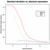
Figure 1
Figure 1
The smooth curves shown were fitted to the scatter plots of SD versus average of log (base 2) expression for each gene using MAS 5.0, dChip and RMA on the dilution data. All genes for all six concentrations in liver and CNS groups were used.
Figure 2
Figure 2
(A) Log (base 2) fold change estimates of gene expression between liver and CNS samples computed from arrays hybridized to 1.25 µg of cRNA using MAS 5.0 plotted against the same estimates obtained from arrays hybridized to 20 µg. Genes demonstrating 2- to 3-fold inconsistencies are shown with squares. Genes demonstrating inconsistencies larger than 3-fold are shown with circles. (B) As (A) but using dChip. (C) As (A) but using RMA.
Figure 2
Figure 2
(A) Log (base 2) fold change estimates of gene expression between liver and CNS samples computed from arrays hybridized to 1.25 µg of cRNA using MAS 5.0 plotted against the same estimates obtained from arrays hybridized to 20 µg. Genes demonstrating 2- to 3-fold inconsistencies are shown with squares. Genes demonstrating inconsistencies larger than 3-fold are shown with circles. (B) As (A) but using dChip. (C) As (A) but using RMA.
Figure 3
Figure 3
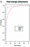
(Previous page and above) ROC curves for spike-in experiments. (A) For 10 pairs of arrays, chosen at random from the Affymetrix spike-in experiment, true positive rates (sensitivity) are estimated for the filtering operation, Observed Fold Change > cut-off, for a large range of cut-off values, by calculating the proportion of genes spiked-in at different concentrations that satisfy the filtering criterion. False positive rates (1 – specificity) are calculated in a similar way by computing the proportion of non-spiked-in genes, which satisfy the filtering criteria. (B) As (A) but using the GeneLogic spike-in experiment. (C) As (A) but selecting 10 comparisons for which the fold changes of spike-in concentrations are 2. (D) As (A) but using the filtering operation test statistic > cut-off. We used the software default test statistics for MAS 5.0 and dChip. (E) As (D) but using the GeneLogic spike-in experiment. (F) As (A) but comparing the average fold changes obtained from two sets of 12 replicate arrays.
Figure 3
Figure 3
(Previous page and above) ROC curves for spike-in experiments. (A) For 10 pairs of arrays, chosen at random from the Affymetrix spike-in experiment, true positive rates (sensitivity) are estimated for the filtering operation, Observed Fold Change > cut-off, for a large range of cut-off values, by calculating the proportion of genes spiked-in at different concentrations that satisfy the filtering criterion. False positive rates (1 – specificity) are calculated in a similar way by computing the proportion of non-spiked-in genes, which satisfy the filtering criteria. (B) As (A) but using the GeneLogic spike-in experiment. (C) As (A) but selecting 10 comparisons for which the fold changes of spike-in concentrations are 2. (D) As (A) but using the filtering operation test statistic > cut-off. We used the software default test statistics for MAS 5.0 and dChip. (E) As (D) but using the GeneLogic spike-in experiment. (F) As (A) but comparing the average fold changes obtained from two sets of 12 replicate arrays.
Figure 4
Figure 4
MvA plots (described in the text) for Affymetrix’s spike-in experiment. (A) For MAS 5.0, observed log (base 2) fold change (M) is plotted against average log (base 2) expression (A) for all genes from spike-in experiment array pairs. A reference array was selected from one of the replicate spike-in experiments and compared to all other arrays in that replicate experiment. The colored numbers represent the log (base 2) fold change in concentrations of all 14 spiked-in genes. Each distinct fold change is represented with a different color as a visual aid. The –∞ and ∞ represent fold changes with a zero in the numerator or denominator, respectively. The red points represent non-spiked-in genes with a fold change larger than 2. (B) As (A) but using dChip. (C) As (A) but using RMA.
Figure 4
Figure 4
MvA plots (described in the text) for Affymetrix’s spike-in experiment. (A) For MAS 5.0, observed log (base 2) fold change (M) is plotted against average log (base 2) expression (A) for all genes from spike-in experiment array pairs. A reference array was selected from one of the replicate spike-in experiments and compared to all other arrays in that replicate experiment. The colored numbers represent the log (base 2) fold change in concentrations of all 14 spiked-in genes. Each distinct fold change is represented with a different color as a visual aid. The –∞ and ∞ represent fold changes with a zero in the numerator or denominator, respectively. The red points represent non-spiked-in genes with a fold change larger than 2. (B) As (A) but using dChip. (C) As (A) but using RMA.
Figure 5
Figure 5
Box plots showing the distribution of observed fold changes for non-spiked in genes. The different colors represent the different quantiles. The relationship of color and quantile is demonstrated in the first box from the left.

Similar articles

Cited by

References

    1. Lockhart D., Dong,H., Byrne,M., Follettie,M., Gallo,M., Chee M., Mittmann,M., Wang,C., Kobayashi,M., Horton,H. et al. (1996) Expression monitoring by hybridization to high-density oligonucleotide arrays. Nat. Biotechnol., 14, 1675–1680. - PubMed
    1. Lipshutz R., Fodor,S., Gingeras,T. and Lockhart D. (1999) High density synthetic oligonucleotide arrays. Nature Genet., Suppl. 21, 20–24. - PubMed
    1. Affymetrix (1999) Microarray Suite User Guide, Version 4. Affymetrix, http://www.affymetrix.com/support/technical/manuals.affx.
    1. Irizarry R., Hobbs,B., Collin,F., Beazer-Barclay,Y., Antonellis,K., Scherf,U. and Speed,T. (2003) Exploration, normalization, and summaries of high density oligonucleotide array probe level data. Biostatistics, in press. - PubMed
    1. Affymetrix (2001) Microarray Suite User Guide, Version 5. Affymetrix, http://www.affymetrix.com/support/technical/manuals.affx.

Publication types

MeSH terms

  NODES
twitter 2