Rational inferences about departures from Hardy-Weinberg equilibrium
- PMID: 15834813
- PMCID: PMC1196455
- DOI: 10.1086/430507
Rational inferences about departures from Hardy-Weinberg equilibrium
Abstract
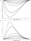
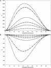
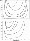
Previous studies have explored the use of departure from Hardy-Weinberg equilibrium (DHW) for fine mapping Mendelian disorders and for general fine mapping. Other studies have used Hardy-Weinberg tests for genotyping quality control. To enable investigators to make rational decisions about whether DHW is due to genotyping error or to underlying biology, we developed an analytic framework and software to determine the parameter values for which DHW might be expected for common diseases. We show analytically that, for a general disease model, the difference between population and Hardy-Weinberg expected genotypic frequencies (delta) at the susceptibility locus is a function of the susceptibility-allele frequency (q), heterozygote relative risk (beta), and homozygote relative risk (gamma). For unaffected control samples, is a function of risk in nonsusceptible homozygotes (alpha), the population prevalence of disease (KP), q, beta, and gamma. We used these analytic functions to calculate and the number of cases or controls needed to detect DHW for a range of genetic models consistent with common diseases (1.1 < or = gamma < or = 10 and 0.005 < or = KP < or = 0.2). Results suggest that significant DHW can be expected in relatively small samples of patients over a range of genetic models. We also propose a goodness-of-fit test to aid investigators in determining whether a DHW observed in the context of a case-control study is consistent with a genetic disease model. We illustrate how the analytic framework and software can be used to help investigators interpret DHW in the context of association studies of common diseases.
Figures




Similar articles
-
Biased tests of association: comparisons of allele frequencies when departing from Hardy-Weinberg proportions.Am J Epidemiol. 1999 Apr 15;149(8):706-11. doi: 10.1093/oxfordjournals.aje.a009878. Am J Epidemiol. 1999. PMID: 10206619
-
Testing Departure from Hardy-Weinberg Proportions.Methods Mol Biol. 2017;1666:83-115. doi: 10.1007/978-1-4939-7274-6_6. Methods Mol Biol. 2017. PMID: 28980243
-
Quantification of the power of Hardy-Weinberg equilibrium testing to detect genotyping error.Hum Hered. 2006;61(1):10-4. doi: 10.1159/000091787. Epub 2006 Mar 1. Hum Hered. 2006. PMID: 16514241
-
[Hardy-Weinberg equilibrium in genetic epidemiology].Zhong Nan Da Xue Xue Bao Yi Xue Ban. 2010 Jan;35(1):90-3. doi: 10.3969/j.issn.1672-7347.2010.01.013. Zhong Nan Da Xue Xue Bao Yi Xue Ban. 2010. PMID: 20130370 Review. Chinese.
-
[Application of chi-square test and exact test in Hardy-Weinberg equilibrium testing].Fa Yi Xue Za Zhi. 2004;20(2):116-9. Fa Yi Xue Za Zhi. 2004. PMID: 15311526 Review. Chinese.
Cited by
-
Genetic predictors of response to serotonergic and noradrenergic antidepressants in major depressive disorder: a genome-wide analysis of individual-level data and a meta-analysis.PLoS Med. 2012;9(10):e1001326. doi: 10.1371/journal.pmed.1001326. Epub 2012 Oct 16. PLoS Med. 2012. PMID: 23091423 Free PMC article.
-
Contribution of the -160C/A polymorphism in the E-cadherin promoter to cancer risk: a meta-analysis of 47 case-control studies.PLoS One. 2012;7(7):e40219. doi: 10.1371/journal.pone.0040219. Epub 2012 Jul 5. PLoS One. 2012. PMID: 22792244 Free PMC article.
-
NCAM1 association study of bipolar disorder and schizophrenia: polymorphisms and alternatively spliced isoforms lead to similarities and differences.Psychiatr Genet. 2007 Apr;17(2):55-67. doi: 10.1097/YPG.0b013e328012d850. Psychiatr Genet. 2007. PMID: 17413444 Free PMC article.
-
Identification of fetal and maternal single nucleotide polymorphisms in candidate genes that predispose to spontaneous preterm labor with intact membranes.Am J Obstet Gynecol. 2010 May;202(5):431.e1-34. doi: 10.1016/j.ajog.2010.03.026. Am J Obstet Gynecol. 2010. PMID: 20452482 Free PMC article.
-
Diplotype trend regression analysis of the ADH gene cluster and the ALDH2 gene: multiple significant associations with alcohol dependence.Am J Hum Genet. 2006 Jun;78(6):973-87. doi: 10.1086/504113. Epub 2006 Apr 11. Am J Hum Genet. 2006. PMID: 16685648 Free PMC article.
References
Electronic-Database Information
-
- DHW software, http://hg-wen.uchicago.edu/dhw2.html
-
- World Health Organization, http://www.who.int/en/
References
-
- Castle WE (1903) The laws of heredity of Galton and Mendel, and some laws governing race improvement by selection. Proc Am Acad Arts Sci 39:223–242
-
- Cramer H (1946) Mathematical methods of statistics. Princeton University Press, Princeton, NJ
-
- Hampe J, Cuthbert A, Croucher PJP, Mirza MM, Mascheretti S, Fischer S, Frenzel H, King K, Hasselmeyer A, MacPherson AJS, Bridger S, van Deventer S, Forbes A, Nikolaus S, Lennard-Jones JE, Foelsch UR, Krawczak M, Lewis C, Schreiber S, Mathew CG (2001) Association between insertion mutation in NOD2 gene and Crohn’s disease in German and British populations. Lancet 357:1925–192810.1016/S0140-6736(00)05063-7 - DOI - PubMed
Publication types
MeSH terms
Substances
Grants and funding
LinkOut - more resources
Full Text Sources

